If you have ever spent twenty minutes adjusting ranges for a VLOOKUP formula, only to drag it down and watch your worksheet fill up with a column of #N/A errors, you are not alone. Even worse is when your spreadsheet freezes entirely, showing a blank screen because you dared to cross-reference lists with more than 10,000 cells. Reconciling tables, cleaning customer email lists, or matching order IDs shouldn’t force you into system crashes or complex scripting.
VLOOKUP (Vertical Lookup) has been the standard way to check worksheets for years, but it is fragile, slow, and structurally limited. When you are reconciling database tables, clean-matching customer email lists, or auditing warehouse stock counts, you need lookup methods that do not crash your system or return false negatives due to simple row offsets.
Here is how you can compare columns using robust, modern spreadsheet techniques without VLOOKUP.
1. The Core Limitations of VLOOKUP
To stop using VLOOKUP, it helps to understand why it fails so frequently during operations:
[Directional Limitations of VLOOKUP]
Lookup Array: [Column B]  <───  Cannot Search Left  <─── [Search Range: Column A]
Lookup Array: [Column A] ───> Searches Right ───> [Search Range: Column B]- The Left-Side Lockout:
VLOOKUPonly searches from left to right. If Column A contains your search query, your lookup reference must exist in Column B or further to the right. If it is located to the left, the formula fails unless you create helper columns or write complexCHOOSEarrays. - Linear Recalculation ($O(N)$ Complexity):
VLOOKUPscans worksheets line-by-line. If you cross-reference a list of 20,000 customer contacts against another list of 20,000 rows, Excel has to run up to 400,000,000 checks. This linear process is why spreadsheets freeze under load. - Mismatched References: If you delete or insert a column inside your search index range, the hardcoded column index number in your formula (e.g.,
3) will shift. The formula won’t alert you; it will simply display data from the wrong column.
2. Row-by-Row Matching (For Sorted Lists)
If you have two columns sorted in the exact same order and simply need to verify that row 5 in Column A matches row 5 in Column B, you can use basic logical operators.
Scenario: Reconciling Physical Stock Counts
Imagine you are comparing physical warehouse inventory sheets (Column A) against the system’s ledger export (Column B). The SKU order is identical, and you want to flag count mismatches:
| Row | Col A (Physical SKU) | Col B (System SKU) | Formula Result (=A2=B2) | Formula Result (=EXACT(A2,B2)) |
|---|---|---|---|---|
| 2 | SKU-884-RED | SKU-884-RED | TRUE | TRUE |
| 3 | SKU-901-BLU | sku-901-blu | TRUE (Case-Insensitive) | FALSE (Capitalization Mismatch) |
| 4 | SKU-112-BLK | SKU-112-WHT | FALSE (Mismatch) | FALSE |
The Boolean Comparison (=)
To quickly test if two cells match, write this in cell C2:
=A2=B2Drag this formula down the column. Excel returns TRUE if the cells contain matching strings or values and FALSE if they do not. Note that this basic comparison ignores differences in case.
Case-Sensitive Matches (EXACT)
If your SKUs or product codes use case-sensitive formatting (where SKU-901-BLU and sku-901-blu represent different items), standard checks will miss the difference. Use the EXACT function instead:
=EXACT(A2, B2)This formula returns TRUE only if characters and capitalization match exactly.
Custom Labels (IF)
If you want to display descriptive status flags to filter through later, use an IF statement:
=IF(A2=B2, "Match", "Mismatch")3. Set-Based Comparison (For Disordered Columns)
In most real-world scenarios, columns are not sorted in the same order. If you compare them row-by-row, the moment one list has an extra or missing row, the offset will cause every subsequent row to flag as a mismatch.
To prevent this, you need a formula that checks if a value in Column A exists anywhere in Column B, regardless of its row position.
The COUNTIF Method
The COUNTIF formula counts how many times a lookup value appears in a target column.
=IF(COUNTIF($B:$B, A2) > 0, "Matches", "Missing")[COUNTIF Scan Logic]
For each item in Column A (A2) ──> Scan entire column range ($B:$B) ──> Count matches.
If count > 0 ──> Output: "Matches"
If count = 0 ──> Output: "Missing"- How it works:
COUNTIF($B:$B, A2)scans the entirety of Column B. If it counts one or more matches for A2, the formula returns “Matches”. If the count is zero, it returns “Missing”. - The Problem:
COUNTIFscans the entire range even after it finds a match to calculate the total count. This makes it inefficient for large datasets.
The High-Performance MATCH Alternative
For large lists (5,000+ rows), combining ISNUMBER with MATCH is much faster and keeps your sheets running smoothly:
=IF(ISNUMBER(MATCH(A2, $B:$B, 0)), "Matches", "Missing")- How it works:
MATCH(A2, $B:$B, 0)searches Column B for the value in A2. The0parameter requires an exact match. If it finds the value, it returns its row number. If it doesn’t, it returns#N/A. TheISNUMBERwrapper converts the row number toTRUEand errors toFALSE. - Performance Advantage: Unlike
COUNTIF,MATCHterminates its search the instant it finds its first hit, saving processing time on large files.
Scenario: Cleaning Email Opt-Out Lists
Imagine Column A is your master list of 30,000 newsletter subscriber emails. Column B is your CRM unsubscribe log of 5,000 emails. By writing the ISNUMBER + MATCH formula in Column C, you can flag and filter out users who have opted out before your next campaign run.
4. Modern Lookups (Excel 365 & 2021+)
If you are using modern versions of Excel (Office 365 or standalone 2021+), you have access to XLOOKUP, which is designed to replace VLOOKUP entirely.
The XLOOKUP Method
XLOOKUP searches for a value in one range and returns a corresponding value from another range, allowing you to search in any direction.
=XLOOKUP(A2, $B$2:$B$100, $B$2:$B$100, "Missing")If XLOOKUP finds the lookup target in Column B, it returns the target; if it fails, it returns the text defined in the fourth parameter (e.g., “Missing”).
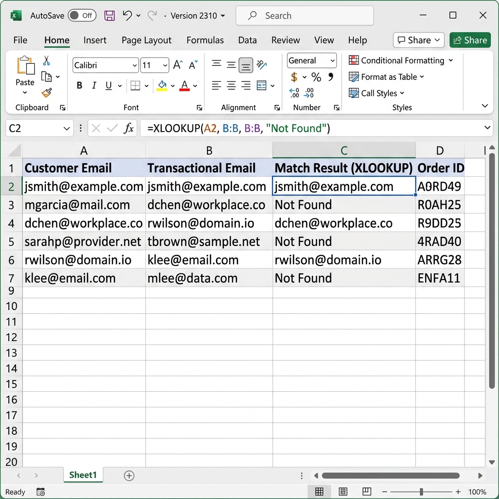 Figure 1: Reconciling customer emails across lists using the XLOOKUP function inside Microsoft Excel.
5. Highlight Matches & Differences Visually
If you need to quickly audit two columns without adding formulas to your sheet, you can use Conditional Formatting to highlight matches or differences.
Method A: Highlight Matches (Duplicates)
This highlights every value in Column A that has a match in Column B.
- Select the data ranges in both columns (e.g. highlight
A2:A100andB2:B100). - Go to the Home tab, click Conditional Formatting > Highlight Cells Rules > Duplicate Values….
- Select Duplicate in the dropdown menu and set your format color (e.g. light green).
- Click OK. All matching values will be highlighted.
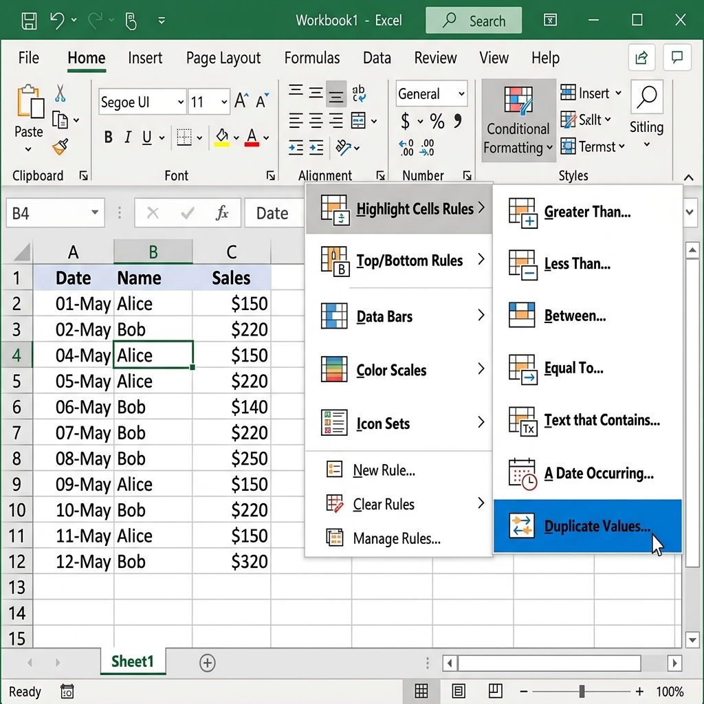 Figure 2: Accessing the Duplicate Values tool through the Conditional Formatting menu in Microsoft Excel.
Method B: Highlight Mismatches (Unique Values)
If you want to highlight values in Column A that are missing from Column B:
- Select only the data in Column A (e.g.
A2:A100). - Go to Home > Conditional Formatting > New Rule.
- Select Use a formula to determine which cells to format.
- Enter the following formula:
=COUNTIF($B$2:$B$100, A2)=0 - Click Format, select a fill color (e.g. light red), and click OK.
6. Secure, Local-First Browser Alternatives
While formulas and formatting are useful, Excel starts to struggle when you need to match and reconcile complex lists from different sources (like CSV logs, system lists, or database outputs).
Many users turn to online converters or web-based diff checkers to speed up the process. However, this introduces serious security risks.
   Data Security Path Analysis

   Cloud-Based Comparison Tools:
   [Spreadsheet Data] ──(Network Transmission)──> [Cloud Server] ──> [Database Logs]

   Local-First Web Tools (FixData):
   [Spreadsheet Data] ──(Local Clipboard Copy)──> [In-Browser Web Worker] ──> [Safe Deletion]
The Risks of Cloud Uploads
Uploading spreadsheets containing customer lists, email addresses, order IDs, or financial records to external servers runs the risk of data leaks and compliance violations. Under GDPR, HIPAA, and standard corporate security policies, transmitting unencrypted client identifiers is a high-risk activity that can lead to audit failures or penalties.
The Local-First Solution
If you need to compare datasets quickly and securely, FixData offers a browser-based alternative that processes everything locally:
- 100% Client-Side Processing: All list hashing, set comparisons, and line cleanups execute directly in your browser’s sandboxed memory. No files are uploaded to external servers, and no data leaves your device.
- Asynchronous Web Workers: FixData runs comparison engines on a background browser thread. This prevents your browser window from freezing even when comparing datasets with over 100,000 lines.
- One-Click Formatting Cleanup: Copy-pasting data between different systems often introduces hidden formatting errors like trailing spaces, carriage returns, or invisible Unicode characters. FixData scans and cleans these formatting anomalies automatically with a single click.
7. Column Comparison Methods Reference
| Method | Best For | Max Data Size | Directional Limit | Case-Sensitive Option |
|---|---|---|---|---|
=A2=B2 | Side-by-side matches | Small (<5k rows) | Row-by-row only | Yes (Via EXACT) |
COUNTIF | Simple presence checks | Medium (<20k rows) | None | No |
ISNUMBER + MATCH | Disordered column matching | Large (50k+ rows) | None | No |
XLOOKUP | Office 365 dynamic search | Large (100k+ rows) | None | No |
| Conditional Formatting | Quick visual audits | Medium (<20k rows) | None | No |
| FixData (Local-First) | High-speed, private lists | Unlimited (Web Workers) | None | Yes (Toggleable settings) |
FAQ Section
Why does Excel flag two identical-looking cells as mismatches?
This is usually caused by hidden characters like trailing spaces, different cell formatting, or carriage returns. Ensure you clean your columns using search-and-replace to strip blank spaces, or use the automatic sanitization options on FixData.
Does MATCH look left in Excel?
Yes. Unlike VLOOKUP, the MATCH function search is directional-independent because it only looks for the value’s index, not a column coordinate to the right.
Can Excel handle comparing two lists of 200,000 rows?
Excel can process large comparisons, but complex formulas like COUNTIF or heavy conditional formatting on hundreds of thousands of cells will likely freeze the application. For large files, it is best to use a tool that supports browser-based multi-threading or database queries.
Action Checklist for Operations Teams
- Identify sorting status: Are your columns in the same row order? If not, skip
A2=B2and useMATCHorXLOOKUP. - Check file size: If your sheets exceed 20,000 rows, avoid
COUNTIFto keep recalculation speeds fast. - Review compliance standards: If your columns contain customer emails, IDs, or financial records, do not upload them to external cloud file converters.
- Clean formatting anomalies: Before running a comparison, run a sweep to strip trailing spaces and hidden carriage returns.
Author Section
Written by FixData Team
We build privacy-first spreadsheet comparison, data reconciliation, and Excel workflow tools designed to help teams compare, clean, and validate data without uploading files to external servers.